Project: Predicting Ad clicks
In this project, we are going to use this dataset from Kaggle. We will be modeling whether a user is going to click on an Ad or not based on the given features.
Highlights:
- Exploratory data analysis
- Defining pipeline
- Logistic regression model
- Cross validation scores
- XGBoost Classifier model
- XGBoost Randomforest model
#Necessary imports
import numpy as np
import pandas as pd
#Visualization libraries
import matplotlib.pyplot as plt
import seaborn as  sns
%matplotlib inline
sns.set()
#Read dataset
advert = pd.read_csv('advertisiment.csv')
#glimpse of data
advert.head(3)
| Daily Time Spent on Site | Age | Area Income | Daily Internet Usage | Ad Topic Line | City | Male | Country | Timestamp | Clicked on Ad | |
|---|---|---|---|---|---|---|---|---|---|---|
| 0 | 68.95 | 35 | 61833.90 | 256.09 | Cloned 5thgeneration orchestration | Wrightburgh | 0 | Tunisia | 2016-03-27 00:53:11 | 0 |
| 1 | 80.23 | 31 | 68441.85 | 193.77 | Monitored national standardization | West Jodi | 1 | Nauru | 2016-04-04 01:39:02 | 0 |
| 2 | 69.47 | 26 | 59785.94 | 236.50 | Organic bottom-line service-desk | Davidton | 0 | San Marino | 2016-03-13 20:35:42 | 0 |
#Information about data
advert.info()

    <class 'pandas.core.frame.DataFrame'>
    RangeIndex: 1000 entries, 0 to 999
    Data columns (total 10 columns):
    Daily Time Spent on Site    1000 non-null float64
    Age                         1000 non-null int64
    Area Income                 1000 non-null float64
    Daily Internet Usage        1000 non-null float64
    Ad Topic Line               1000 non-null object
    City                        1000 non-null object
    Male                        1000 non-null int64
    Country                     1000 non-null object
    Timestamp                   1000 non-null object
    Clicked on Ad               1000 non-null int64
    dtypes: float64(3), int64(3), object(4)
    memory usage: 78.2+ KB
Observation:
- We have both numerical and non-numerical columns to deal with
#Describe numerical features
advert.describe()
| Daily Time Spent on Site | Age | Area Income | Daily Internet Usage | Male | Clicked on Ad | |
|---|---|---|---|---|---|---|
| count | 1000.000000 | 1000.000000 | 1000.000000 | 1000.000000 | 1000.000000 | 1000.00000 |
| mean | 65.000200 | 36.009000 | 55000.000080 | 180.000100 | 0.481000 | 0.50000 |
| std | 15.853615 | 8.785562 | 13414.634022 | 43.902339 | 0.499889 | 0.50025 |
| min | 32.600000 | 19.000000 | 13996.500000 | 104.780000 | 0.000000 | 0.00000 |
| 25% | 51.360000 | 29.000000 | 47031.802500 | 138.830000 | 0.000000 | 0.00000 |
| 50% | 68.215000 | 35.000000 | 57012.300000 | 183.130000 | 0.000000 | 0.50000 |
| 75% | 78.547500 | 42.000000 | 65470.635000 | 218.792500 | 1.000000 | 1.00000 |
| max | 91.430000 | 61.000000 | 79484.800000 | 269.960000 | 1.000000 | 1.00000 |
Observations:
- Males and females seem to be almost even
- Seems like we would have to include all of these features in our prediction
#Describe non-numerical features
advert.describe(include=['O'])
| Ad Topic Line | City | Country | Timestamp | |
|---|---|---|---|---|
| count | 1000 | 1000 | 1000 | 1000 |
| unique | 1000 | 969 | 237 | 1000 |
| top | Multi-layered tangible portal | Lisamouth | Czech Republic | 2016-01-10 23:14:30 |
| freq | 1 | 3 | 9 | 1 |
Observations:
- No feature seems to be worth adding in our prediction model. All will be dropped.
#Lets drop non-numerical features
advert = advert.select_dtypes(exclude='object')
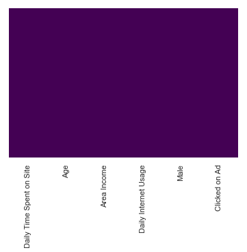
#Check for null values in dataset
sns.heatmap(advert.isnull(),cmap='viridis',cbar=False,yticklabels=False)

    <matplotlib.axes._subplots.AxesSubplot at 0x16797fd3dd8>
#Another way to check for null values in dataset
[col for col in advert.columns if advert[col].isnull().any()]

    []
Looks like there are no null values. Makes our life easier :)
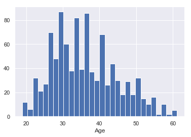
Exploratory data analysis
advert['Age'].hist(bins=30)
plt.xlabel('Age')

    Text(0.5, 0, 'Age')
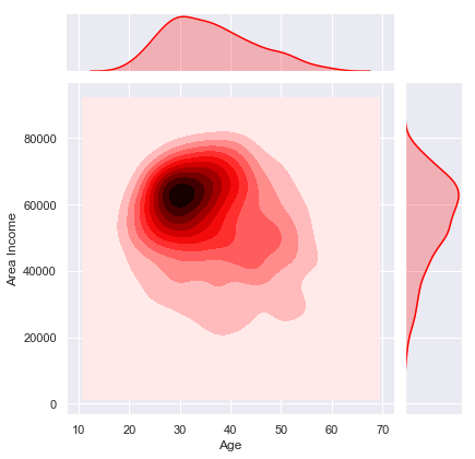
sns.jointplot(x='Age',y='Area Income',data=advert,kind='kde',color='red')

    <seaborn.axisgrid.JointGrid at 0x16798305ac8>
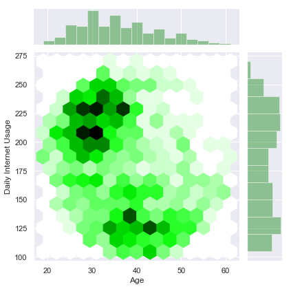
sns.jointplot('Age','Daily Internet Usage',advert,kind='hex',color='green')

    <seaborn.axisgrid.JointGrid at 0x16798422e80>
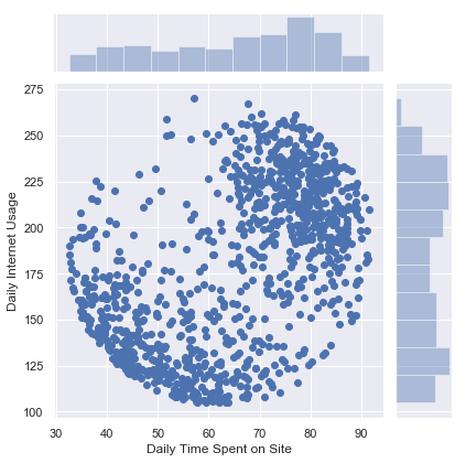
sns.jointplot(x='Daily Time Spent on Site',y='Daily Internet Usage',data=advert)

    <seaborn.axisgrid.JointGrid at 0x1679a61ce80>
sns.countplot(x='Male',hue='Clicked on Ad',data=advert)
plt.legend(bbox_to_anchor=(1.05, 1), loc=2, borderaxespad=0.)

    <matplotlib.legend.Legend at 0x1679a71f588>
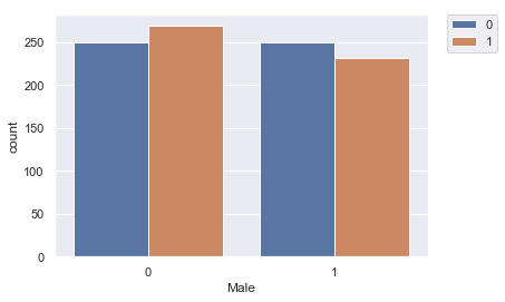
Male feature is not the perfect predictor of our target.
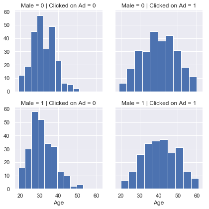
g = sns.FacetGrid(data=advert,row='Male',col='Clicked on Ad')
g.map(plt.hist,'Age')

    <seaborn.axisgrid.FacetGrid at 0x1679a78f748>
g = sns.FacetGrid(data=advert,row='Male',col='Clicked on Ad')
g.map(plt.hist,'Daily Internet Usage')

    <seaborn.axisgrid.FacetGrid at 0x16798422ba8>
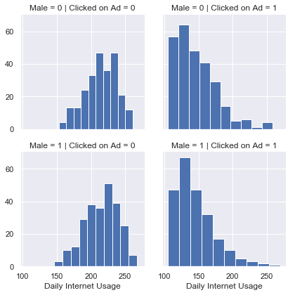
Seems like people with less internet usage have more click through rate.
Define Pipeline
from sklearn.pipeline import make_pipeline
from sklearn.linear_model import LogisticRegression
X = advert.drop('Clicked on Ad',axis=1)
y = advert['Clicked on Ad']
my_pipeline = make_pipeline(LogisticRegression(solver='liblinear'))
Cross validation scores
from sklearn.model_selection import cross_val_score
cross_scores = cross_val_score(my_pipeline,X,y,cv=5,scoring='accuracy')
cross_scores.mean()

    0.8959999999999999
We got a pretty good model, as our accuracy score is 89%.
Using XGBoost
from xgboost import XGBClassifier,XGBRFClassifier
from sklearn.model_selection import train_test_split
X_train, X_valid, y_train, y_valid = train_test_split(X, y, test_size=0.2, random_state=1)
model =XGBClassifier(n_estimators=1000,learning_rate=0.05,n_jobs=4)
model.fit(X_train,y_train,early_stopping_rounds=5,eval_set=[(X_valid,y_valid)],verbose=False)

    XGBClassifier(base_score=0.5, booster='gbtree', colsample_bylevel=1,
           colsample_bynode=1, colsample_bytree=1, gamma=0, gpu_id=-1,
           importance_type='gain', interaction_constraints='',
           learning_rate=0.05, max_delta_step=0, max_depth=6,
           min_child_weight=1, missing=nan, monotone_constraints='()',
           n_estimators=1000, n_jobs=4, num_parallel_tree=1,
           objective='binary:logistic', random_state=0, reg_alpha=0,
           reg_lambda=1, scale_pos_weight=1, subsample=1, tree_method='exact',
           validate_parameters=1, verbosity=None)
predictions = model.predict(X_valid)
from sklearn.metrics import accuracy_score,confusion_matrix,classification_report
accuracy_score(y_valid,predictions)

    0.94
print(classification_report(y_valid,predictions))

                  precision    recall  f1-score   support

               0       0.90      0.99      0.94       103
               1       0.99      0.89      0.93        97

       micro avg       0.94      0.94      0.94       200
       macro avg       0.95      0.94      0.94       200
    weighted avg       0.94      0.94      0.94       200
Great, using XGBoost classifier, we were able to achieve 94% accuracy. Let us now test using the RandomForest flavor of XGBoost.
model = XGBRFClassifier (n_estimators=1000,learning_rate=0.05,n_jobs=4)
model.fit(X_train,y_train,early_stopping_rounds=5,eval_set=[(X_valid,y_valid)],verbose=False)

    XGBRFClassifier(base_score=0.5, booster='gbtree', colsample_bylevel=1,
            colsample_bynode=0.8, colsample_bytree=1, gamma=0, gpu_id=-1,
            importance_type='gain', interaction_constraints='',
            learning_rate=0.05, max_delta_step=0, max_depth=6,
            min_child_weight=1, missing=nan, monotone_constraints='()',
            n_estimators=1000, n_jobs=4, num_parallel_tree=1000,
            objective='binary:logistic', random_state=0, reg_alpha=0,
            reg_lambda=1e-05, scale_pos_weight=1, subsample=0.8,
            tree_method='exact', validate_parameters=1, verbosity=None)
predictions = model.predict(X_valid)
accuracy_score(y_valid,predictions)

    0.96
print(classification_report(y_valid,predictions))

                  precision    recall  f1-score   support

               0       0.93      1.00      0.96       103
               1       1.00      0.92      0.96        97

       micro avg       0.96      0.96      0.96       200
       macro avg       0.96      0.96      0.96       200
    weighted avg       0.96      0.96      0.96       200
Awesome, we were able to achieve even better results on this.
Leave a comment