Project: Predicting Amount spent

For this project, we are going to use this dataset from Kaggle. This data is of ecommerce customers and their usage on app vs website. Our mission is to comeup with a model that will predict the ‘Yearly Amount Spent’ by the customers based on the given features.

Highlights:

• Exploratory data analysis
• Creating pipeline
• Using LinearRegression model
• Using cross-validation scores to measure model performance

#Imports
import numpy as np
import pandas as pd

#Visualization imports
import matplotlib.pyplot as plt
import seaborn as sns

%matplotlib inline
sns.set()

#import data
ecommerce = pd.read_csv('ecommerce')

#Glimpse of data
ecommerce.head(2)

	Email	Address	Avatar	Avg. Session Length	Time on App	Time on Website	Length of Membership	Yearly Amount Spent
0	mstephenson@fernandez.com	835 Frank Tunnel\nWrightmouth, MI 82180-9605	Violet	34.497268	12.655651	39.577668	4.082621	587.951054
1	hduke@hotmail.com	4547 Archer Common\nDiazchester, CA 06566-8576	DarkGreen	31.926272	11.109461	37.268959	2.664034	392.204933

#Data info
ecommerce.info()

    <class 'pandas.core.frame.DataFrame'>
    RangeIndex: 500 entries, 0 to 499
    Data columns (total 8 columns):
    Email                   500 non-null object
    Address                 500 non-null object
    Avatar                  500 non-null object
    Avg. Session Length     500 non-null float64
    Time on App             500 non-null float64
    Time on Website         500 non-null float64
    Length of Membership    500 non-null float64
    Yearly Amount Spent     500 non-null float64
    dtypes: float64(5), object(3)
    memory usage: 31.3+ KB

#describe numerical features
ecommerce.describe()

	Avg. Session Length	Time on App	Time on Website	Length of Membership	Yearly Amount Spent
count	500.000000	500.000000	500.000000	500.000000	500.000000
mean	33.053194	12.052488	37.060445	3.533462	499.314038
std	0.992563	0.994216	1.010489	0.999278	79.314782
min	29.532429	8.508152	33.913847	0.269901	256.670582
25%	32.341822	11.388153	36.349257	2.930450	445.038277
50%	33.082008	11.983231	37.069367	3.533975	498.887875
75%	33.711985	12.753850	37.716432	4.126502	549.313828
max	36.139662	15.126994	40.005182	6.922689	765.518462

Observation:

• Our features seem to be normally distributed as mean is very close to median values
• The feature data is spread very close to the mean as standard deviation is very low

#Drop the non-numerical columns
ecommerce.drop(['Address','Avatar','Email'],axis=1,inplace=True)

#Check for null values
[col for col in ecommerce.columns if ecommerce[col].isnull().any()]

    []

Seems like there are no null values. Makes our life easier :)

Exploratory data analysis

Let’s explore our data a bit

sns.distplot(ecommerce['Avg. Session Length'],label='Avg. session length')
sns.distplot(ecommerce['Time on App'],label='Time on app')
sns.distplot(ecommerce['Time on Website'],label='Time on Website')
sns.distplot(ecommerce['Length of Membership'],label='Length of membership')
plt.legend()
plt.legend(bbox_to_anchor=(1.05, 1), loc=2, borderaxespad=0.)

    <matplotlib.legend.Legend at 0x167f8cb3c50>

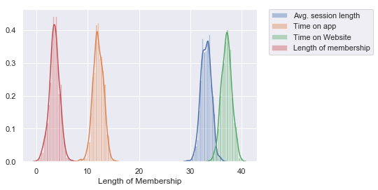
Distribution plot above proves our first observation that features are normally distributed.

plt.figure(figsize=(10,5))
sns.boxenplot(data=ecommerce.drop('Yearly Amount Spent',axis=1))
plt.tight_layout()

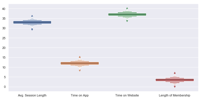
Above Boxplot proves our second observation that the features data spread is very close to the mean.

#Pair plot
sns.pairplot(ecommerce)

    <seaborn.axisgrid.PairGrid at 0x167fb0f9a58>

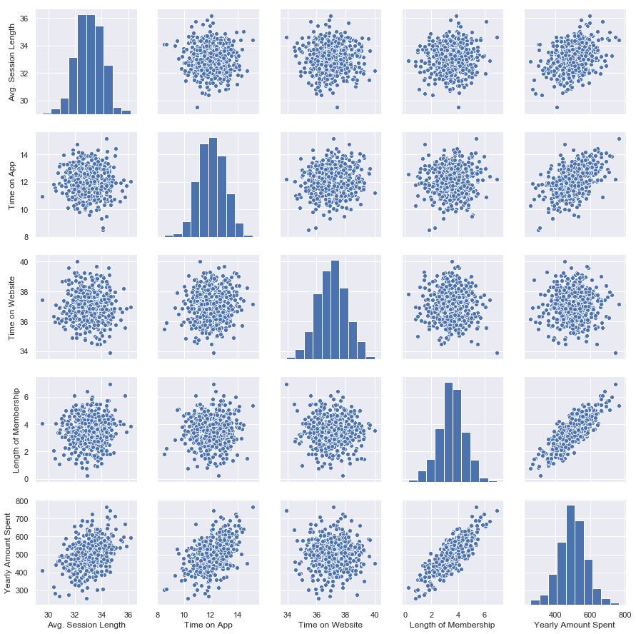
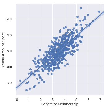
There seems to be a very strong relationship b/w length of membership and our target label.

sns.heatmap(ecommerce.corr(),cmap='magma_r',annot=True)

    <matplotlib.axes._subplots.AxesSubplot at 0x167fbcf1748>

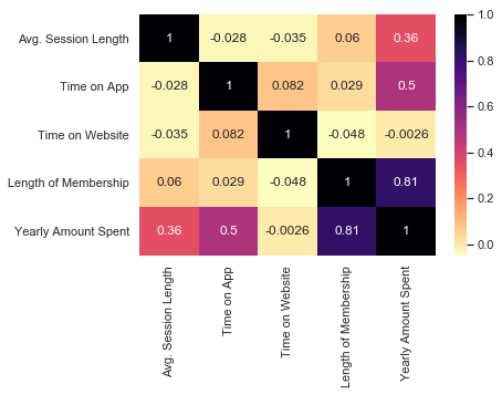
Heatmap proves that relationship by showing us the pearson’s r value of 0.81. There also seems to be some relation between Time on App and our target variable.

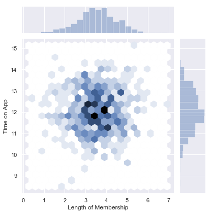
sns.jointplot(x='Length of Membership',y='Time on App',data=ecommerce,kind='hex')

    <seaborn.axisgrid.JointGrid at 0x167fc21a940>

sns.lmplot(x='Length of Membership',y='Yearly Amount Spent',data=ecommerce)

    <seaborn.axisgrid.FacetGrid at 0x167fc7c0668>

Defining pipeline

X = ecommerce.drop('Yearly Amount Spent',axis=1)
y = ecommerce['Yearly Amount Spent']

from sklearn.linear_model import LinearRegression
from sklearn.pipeline import make_pipeline

my_pipeline = make_pipeline(LinearRegression())

Using cross-validation scores

from sklearn.model_selection import cross_val_score

cv_scores = -1 * cross_val_score(my_pipeline,X,y,cv=5,scoring='neg_mean_absolute_error')

cv_scores.mean()

    7.944690345653413