Project: Analyzing Stocks
In this project, we will focus on exploratory data analysis of stock prices for following companies from 2006 to 2015.
- Amazon
- Microsoft
- Bank of America
- Citibank
#Imports
import numpy as np
import pandas as pd
import pandas_datareader.data as web
import datetime as dt
#visualization libraries
import matplotlib.pyplot as plt
import seaborn as sns
#Start and end period
start = dt.datetime(2006,1,1)
end = dt.datetime(2016,1,1)
#Tickers of the companies
tickers = ['AMZN','MSFT','BAC','C']
#Fetch data from yahoo stocks using DataReader
amazon = web.DataReader('AMZN',data_source='yahoo',start=start,end=end)
microsoft = web.DataReader('MSFT',data_source='yahoo',start=start,end=end)
bank_of_america = web.DataReader('BAC',data_source='yahoo',start=start,end=end)
citigroup = web.DataReader('C',data_source='yahoo',start=start,end=end)
#Concating all the data frames of different companies into one large data frame.
stock_data = pd.concat([amazon,microsoft,bank_of_america,citigroup],axis=1,keys=tickers)
#Adding column names
stock_data.columns.names = ['Tickers','Stock Info']
#Glimpse of data
stock_data.head()
| Tickers | AMZN | MSFT | BAC | C | ||||||||||||||||||||
|---|---|---|---|---|---|---|---|---|---|---|---|---|---|---|---|---|---|---|---|---|---|---|---|---|
| Stock Info | High | Low | Open | Close | Volume | Adj Close | High | Low | Open | Close | Volume | Adj Close | High | Low | Open | Close | Volume | Adj Close | High | Low | Open | Close | Volume | Adj Close |
| Date | ||||||||||||||||||||||||
| 2006-01-03 | 47.849998 | 46.250000 | 47.470001 | 47.580002 | 7582200 | 47.580002 | 27.000000 | 26.10 | 26.250000 | 26.840000 | 79973000.0 | 19.602528 | 47.180000 | 46.150002 | 46.919998 | 47.080002 | 16296700.0 | 35.298687 | 493.799988 | 481.100006 | 490.000000 | 492.899994 | 1537600.0 | 440.882477 |
| 2006-01-04 | 47.730000 | 46.689999 | 47.490002 | 47.250000 | 7440900 | 47.250000 | 27.080000 | 26.77 | 26.770000 | 26.969999 | 57975600.0 | 19.697485 | 47.240002 | 46.450001 | 47.000000 | 46.580002 | 17757900.0 | 34.923801 | 491.000000 | 483.500000 | 488.600006 | 483.799988 | 1870900.0 | 432.742950 |
| 2006-01-05 | 48.200001 | 47.110001 | 47.160000 | 47.650002 | 5417200 | 47.650002 | 27.129999 | 26.91 | 26.959999 | 26.990000 | 48245500.0 | 19.712091 | 46.830002 | 46.320000 | 46.580002 | 46.639999 | 14970700.0 | 34.968796 | 487.799988 | 484.000000 | 484.399994 | 486.200012 | 1143100.0 | 434.889679 |
| 2006-01-06 | 48.580002 | 47.320000 | 47.970001 | 47.869999 | 6152900 | 47.869999 | 27.000000 | 26.49 | 26.889999 | 26.910000 | 100963000.0 | 19.653666 | 46.910000 | 46.349998 | 46.799999 | 46.570000 | 12599800.0 | 34.916302 | 489.000000 | 482.000000 | 488.799988 | 486.200012 | 1370200.0 | 434.889679 |
| 2006-01-09 | 47.099998 | 46.400002 | 46.549999 | 47.080002 | 8943100 | 47.080002 | 27.070000 | 26.76 | 26.930000 | 26.860001 | 55625000.0 | 19.617136 | 46.970001 | 46.360001 | 46.720001 | 46.599998 | 15619400.0 | 34.938789 | 487.399994 | 483.000000 | 486.000000 | 483.899994 | 1680700.0 | 432.832489 |
#Max close price for each company's stock
stock_data.xs(key='Close',level='Stock Info',axis=1).max()

    Tickers
    AMZN    693.969971
    MSFT     56.549999
    BAC      54.900002
    C       564.099976
    dtype: float64
#Return of each company
returns = pd.DataFrame()
for ticker in tickers:
    returns[ticker] = stock_data[ticker]['Close'].pct_change()
returns.head()
| AMZN | MSFT | BAC | C | |
|---|---|---|---|---|
| Date | ||||
| 2006-01-03 | NaN | NaN | NaN | NaN |
| 2006-01-04 | -0.006936 | 0.004843 | -0.010620 | -0.018462 |
| 2006-01-05 | 0.008466 | 0.000742 | 0.001288 | 0.004961 |
| 2006-01-06 | 0.004617 | -0.002964 | -0.001501 | 0.000000 |
| 2006-01-09 | -0.016503 | -0.001858 | 0.000644 | -0.004731 |
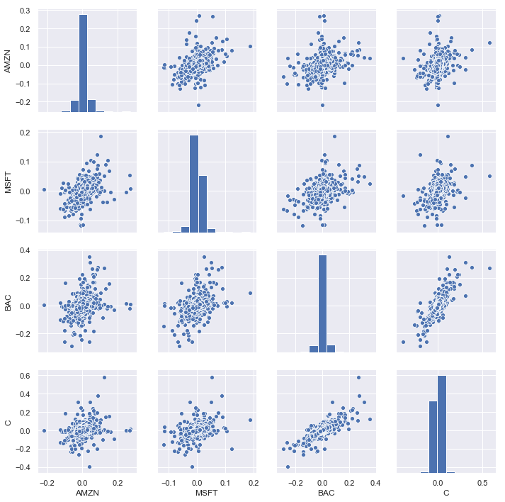
sns.pairplot(returns)

    <seaborn.axisgrid.PairGrid at 0x1877dbb83c8>
#Worst return date for each company
returns.idxmin()

    AMZN   2006-07-26
    MSFT   2009-01-22
    BAC    2009-01-20
    C      2009-02-27
    dtype: datetime64[ns]
#Best return date for each company
returns.idxmax()

    AMZN   2007-04-25
    MSFT   2008-10-13
    BAC    2009-04-09
    C      2008-11-24
    dtype: datetime64[ns]
#Standard deviation of returns
returns.std()

    AMZN    0.026638
    MSFT    0.017764
    BAC     0.036647
    C       0.038672
    dtype: float64
#Standard deviation of returns for year 2015
returns.loc['2015-01-01':'2015-12-31'].std()

    AMZN    0.021147
    MSFT    0.017801
    BAC     0.016163
    C       0.015289
    dtype: float64
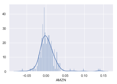
#Lets create distribution plot of the stock returns of Amazon for year 2015
sns.distplot(returns.loc['2015-01-01':'2015-12-31']['AMZN'],bins=100)

    <matplotlib.axes._subplots.AxesSubplot at 0x1877f3e4588>
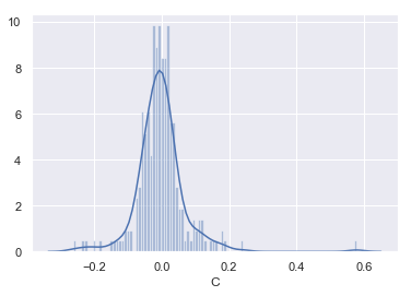
#Lets create distribution plot of the stock returns of Citigroup for year 2008
sns.distplot(returns.loc['2008-01-01':'2008-12-31']['C'],bins=100)

    <matplotlib.axes._subplots.AxesSubplot at 0x187009ce518>
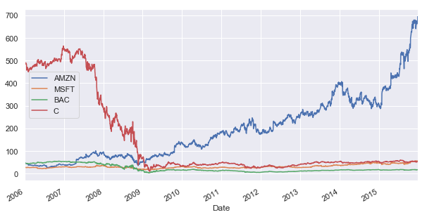
#Close price of each company throughout the entire time period of 2006-2015
stock_data.xs(key='Close',axis=1,level='Stock Info').plot(figsize=(10,5))
plt.legend()

    <matplotlib.legend.Legend at 0x1877fdf1278>
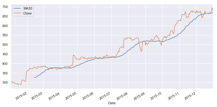
#30 day moving average of Amazon for year 2015
stock_data.loc['2015-1-1':'2015-12-31','AMZN']['Close'].rolling(30).mean().plot(figsize=(10,5),label='MA30')
stock_data.loc['2015-1-1':'2015-12-31','AMZN']['Close'].plot(label='Close')
plt.tight_layout()
plt.legend()

    <matplotlib.legend.Legend at 0x1870483e048>
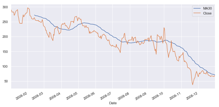
#30 day moving average of Citigroup for year 2008
stock_data.loc['2008-1-1':'2008-12-31','C']['Close'].rolling(30).mean().plot(figsize=(10,5),label='MA30')
stock_data.loc['2008-1-1':'2008-12-31','C']['Close'].plot(label='Close')
plt.tight_layout()
plt.legend()

    <matplotlib.legend.Legend at 0x18704839898>
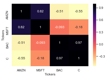
#Heatmap for the relation between close prices of different stocks
sns.heatmap(stock_data.xs(key='Close',axis=1,level='Stock Info').corr(),cmap='magma_r',annot=True)

    <matplotlib.axes._subplots.AxesSubplot at 0x18704ae9a58>
Leave a comment