Project: Predicting Iowa house prices

In this project, we will be predicting the house prices of Iowa houses. Let’s get started
We will be using the steps that were referenced here SML:Supervised Machine Learning workflow
The data set that we are going to use is the Iowa house prices dataset from Kaggle.
Highlights:

• Exploratory data analysis using Pandas
• Visualizing data using matplotlib and seaborn
• Imputing null values
• Training DecisionTreeRegressor and retraining with different max_leaf_nodes values
• Applying the concept of Bias-Variance Tradeoff
• Fitting and validating RandomForestRegressor and comparing the results with that of DecisionTreeRegressor

Define Problem

Since we are to predict the house prices, it is going to be a regression problem.

Acquire Data

Go ahead and download the dataset from the Kaggle link above

Import Data

#Importing necessary libraries
import numpy as np
import pandas as pd

#Visualization libraries
import matplotlib.pyplot as plt
import seaborn as sns

%matplotlib inline
sns.set()

#Reading csv
iowa = pd.read_csv("train.csv")

iowa.head()

	Id	MSSubClass	MSZoning	LotFrontage	LotArea	Street	Alley	LotShape	LandContour	Utilities	...	PoolArea	PoolQC	Fence	MiscFeature	MiscVal	MoSold	YrSold	SaleType	SaleCondition	SalePrice
0	1	60	RL	65.0	8450	Pave	NaN	Reg	Lvl	AllPub	...	0	NaN	NaN	NaN	0	2	2008	WD	Normal	208500
1	2	20	RL	80.0	9600	Pave	NaN	Reg	Lvl	AllPub	...	0	NaN	NaN	NaN	0	5	2007	WD	Normal	181500
2	3	60	RL	68.0	11250	Pave	NaN	IR1	Lvl	AllPub	...	0	NaN	NaN	NaN	0	9	2008	WD	Normal	223500
3	4	70	RL	60.0	9550	Pave	NaN	IR1	Lvl	AllPub	...	0	NaN	NaN	NaN	0	2	2006	WD	Abnorml	140000
4	5	60	RL	84.0	14260	Pave	NaN	IR1	Lvl	AllPub	...	0	NaN	NaN	NaN	0	12	2008	WD	Normal	250000

5 rows × 81 columns

Exploratory Data Analysis

Lets explore our data a bit and see what do we have in hand

len(iowa.columns)
  81

There are 81 columns, for the sake of this project and for understanding purposes, we will use only following features: LotFrontage, LotArea, Utilities, BldgType, HouseStyle, YearBuilt, 1stFlrSF, 2ndFlrSF, BedroomAbvGr, YrSold, SaleType, SalePrice

features = ['LotFrontage','LotArea','Utilities','BldgType','HouseStyle','YearBuilt','1stFlrSF','2ndFlrSF','BedroomAbvGr','YrSold','SaleType']
target = 'SalePrice'
#Feature Dataframe
iowa_feat = iowa[features]
#Target Dataframe
iowa_tar = iowa[target]
iowa = pd.concat([iowa_feat,iowa_tar],axis=1)

iowa_feat.head(3)

	LotFrontage	LotArea	Utilities	BldgType	HouseStyle	YearBuilt	1stFlrSF	2ndFlrSF	BedroomAbvGr	YrSold	SaleType
0	65.0	8450	AllPub	1Fam	2Story	2003	856	854	3	2008	WD
1	80.0	9600	AllPub	1Fam	1Story	1976	1262	0	3	2007	WD
2	68.0	11250	AllPub	1Fam	2Story	2001	920	866	3	2008	WD

#get the idea of number of rows and columns and type of data in each
iowa_feat.info()

    <class 'pandas.core.frame.DataFrame'>
    RangeIndex: 1460 entries, 0 to 1459
    Data columns (total 11 columns):
    LotFrontage     1201 non-null float64
    LotArea         1460 non-null int64
    Utilities       1460 non-null object
    BldgType        1460 non-null object
    HouseStyle      1460 non-null object
    YearBuilt       1460 non-null int64
    1stFlrSF        1460 non-null int64
    2ndFlrSF        1460 non-null int64
    BedroomAbvGr    1460 non-null int64
    YrSold          1460 non-null int64
    SaleType        1460 non-null object
    dtypes: float64(1), int64(6), object(4)
    memory usage: 125.5+ KB

iowa_feat.describe()

	LotFrontage	LotArea	YearBuilt	1stFlrSF	2ndFlrSF	BedroomAbvGr	YrSold
count	1201.000000	1460.000000	1460.000000	1460.000000	1460.000000	1460.000000	1460.000000
mean	70.049958	10516.828082	1971.267808	1162.626712	346.992466	2.866438	2007.815753
std	24.284752	9981.264932	30.202904	386.587738	436.528436	0.815778	1.328095
min	21.000000	1300.000000	1872.000000	334.000000	0.000000	0.000000	2006.000000
25%	59.000000	7553.500000	1954.000000	882.000000	0.000000	2.000000	2007.000000
50%	69.000000	9478.500000	1973.000000	1087.000000	0.000000	3.000000	2008.000000
75%	80.000000	11601.500000	2000.000000	1391.250000	728.000000	3.000000	2009.000000
max	313.000000	215245.000000	2010.000000	4692.000000	2065.000000	8.000000	2010.000000

Observations:

• LotFrontage
  • Has only 1201 values, which means that there are missing values. We will handle that in the next stage
  • Has mean of 70 ft.
  • Has standard deviation of around 24 ft.
  • Max value seems like an outlier as 75% of the data is within 80 ft.
• LotArea
  • Seems to be highly right skewed distribution
  • Max value is definitely an outlier
• YearBuilt
  • Max is 2010 which means either no house was sold after 2010 or the data was only collected upto 2010
• 1stFlrSF
  • Seems to be evenly distributed
• 2ndFlrSF
  • Upto 50% of the data here has 0 value which means that around 50% of the houses are single storey
• BedroomAbvGr
  • Min is 0 rooms
• YrSold
  • Houses were sold from 2006 to 2010

Observing Categorical Variables

iowa_feat.describe(include=['O'])

	Utilities	BldgType	HouseStyle	SaleType
count	1460	1460	1460	1460
unique	2	5	8	9
top	AllPub	1Fam	1Story	WD
freq	1459	1220	726	1267

• Utilities: -Almost all of the houses belong to single category. I don’t see it affecting our house prices. We may drop it in next stage
• BldgType: -Almost 83% of data points fall in a single category here as well. We might drop this column as well
• HouseStyle: -There seems to be somewhat distribution among multiple categories here. We will include this in our predictions
• SaleType: -Almost 80% of data points fall in a single category. We will drop this column as well

Visualizing Data

Here we will visualize our categorical and numerical variables and confirm some of the descriptive observations that we made above

sns.countplot(data=iowa,x='Utilities')
<matplotlib.axes._subplots.AxesSubplot at 0x249df9fff60>

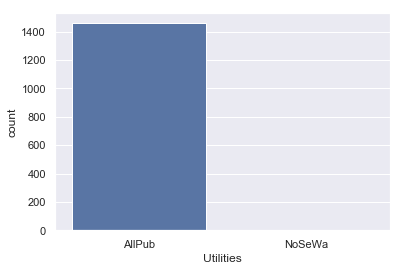
This confirms our above observation that almost all of the data points belong to single category of Utilities

sns.countplot(data=iowa,x='BldgType')
<matplotlib.axes._subplots.AxesSubplot at 0x249df7dff98>

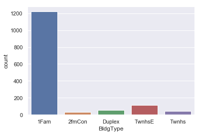
This confirms our observation that ‘BldgType’ doesn’t seem to much impact the target price as well since about 80% of data is in single category. We will drop this also.

sns.countplot(data=iowa,x='HouseStyle')
<matplotlib.axes._subplots.AxesSubplot at 0x249dc69dba8>

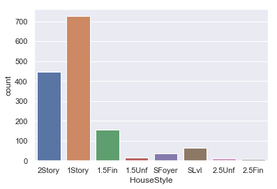
This confirms our observation about ‘HouseStyle’ that there is some distribution here. We will include it in our predictions

sns.countplot(data=iowa,x='SaleType')
<matplotlib.axes._subplots.AxesSubplot at 0x249dc61f390>

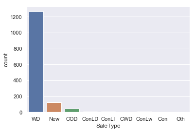
This confirms our observation that almost all of the data points fall under a single category in ‘SaleType’

sns.boxplot(data=iowa,x='LotFrontage',palette='rainbow')
<matplotlib.axes._subplots.AxesSubplot at 0x249df89ff98>

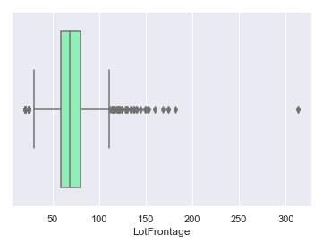
We were right about our observation that 313 is the outlier. Around 50% of data falls between 50 and 100.

plt.figure(figsize=(15,5))
sns.boxplot(data=iowa,x='LotArea',palette='rainbow')
plt.tight_layout()

plt.figure(figsize=(15,5))
sns.distplot(a=iowa['LotArea'],bins=100,kde=False,rug=True)
plt.tight_layout()

Above boxplot and hist plot of ‘LotArea’ confirms our observations that the distribution is highly right skewed. Max value is also an outlier

iowa['1stFlrSF'].plot(kind='hist',bins=30)
<matplotlib.axes._subplots.AxesSubplot at 0x249e513c0f0>

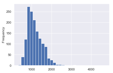
This confirms our observation about ‘1stFlrSF’. The distribution is good. We will include this feature in our predictions

iowa['2ndFlrSF'].plot(kind='hist',bins=30)
<matplotlib.axes._subplots.AxesSubplot at 0x249e4c23c88>

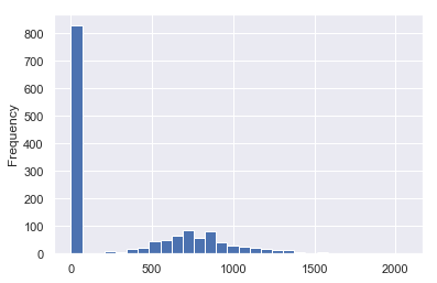
This confirms our observation about ‘2ndFlrSF’. Most of the data points are with 0 value

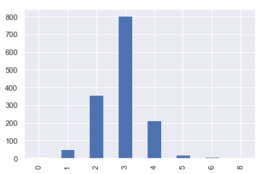
iowa['BedroomAbvGr'].value_counts().sort_index().plot(kind='bar')
<matplotlib.axes._subplots.AxesSubplot at 0x249e50f6e48>

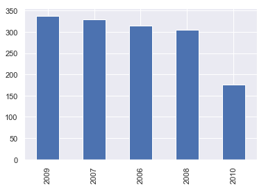
iowa['YrSold'].value_counts().plot(kind='bar')
<matplotlib.axes._subplots.AxesSubplot at 0x249e5382240>

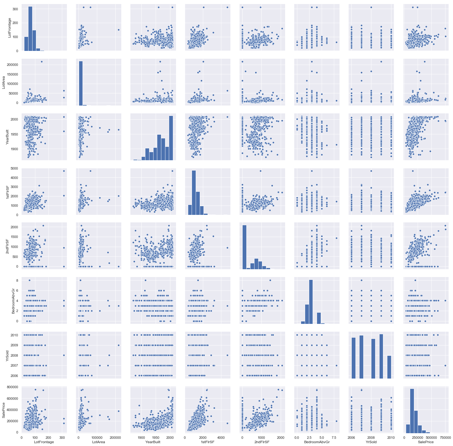
sns.pairplot(data=iowa)
<seaborn.axisgrid.PairGrid at 0x249c7ebcbe0>

sns.heatmap(iowa.corr(),cmap='magma_r',annot=True)
<matplotlib.axes._subplots.AxesSubplot at 0x249eb4f1438>

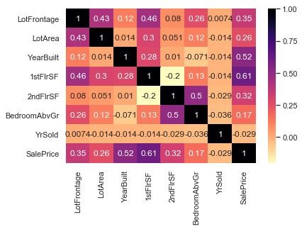
YrSold has almost 0 pearson’s r value in correlation to SalePrice. We will drop this column also.
LotFrontage has some relation to SalePrice, we will keep it and fill it up

Data Cleaning, Data Completing, Feature Engineering

Lets clean the data by dropping the columns we have decided to drop in our above analysis.

iowa_feat.drop(['Utilities','BldgType','SaleType','YrSold'],axis=1,inplace=True)

Lets complete the data now by filling in the null values

#check for null values in our features
plt.figure(figsize=(10,5))
sns.heatmap(iowa_feat.isnull(),cbar=False,yticklabels=False,cmap='viridis')
<matplotlib.axes._subplots.AxesSubplot at 0x249eca01c18>

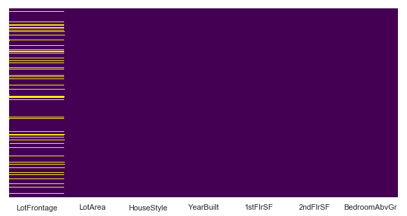
So, only LotFrontage has null values. Lets complete them by filling them with the average value. Do remember that there are alot of ways to fill in the values, but for now, i will just fill them up with the mean value of the column

iowa_feat['LotFrontage'].fillna(iowa_feat['LotFrontage'].mean(),inplace=True)

#check for null values again
plt.figure(figsize=(10,5))
sns.heatmap(iowa_feat.isnull(),cbar=False,yticklabels=False,cmap='viridis')
<matplotlib.axes._subplots.AxesSubplot at 0x249ef63db00>

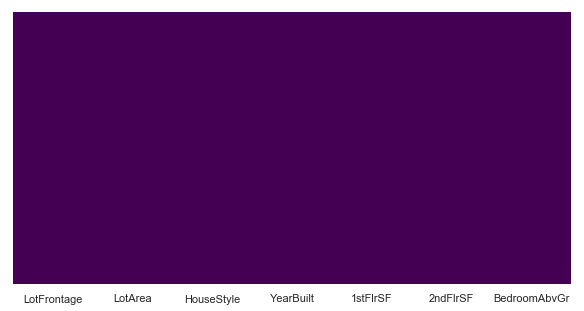
Great, now that we dont have any null values, let’s proceed

Now, we need to convert one of the features to numerical values as part of feature engineering

iowa_feat = pd.get_dummies(iowa_feat,drop_first=True)

Get Model

We will be experimenting with two models in this project, DecisionTreeRegressor and RandomforestTreeRegressor.

from sklearn.tree import DecisionTreeRegressor

dtr = DecisionTreeRegressor()

Train/Fit Model

Now, for this step we need to first split our dataset into training and testing. Note that when you download the dataset from Kaggle, they have done it for you and you won’t have to do it yourself.
But i want to show you how it’s done. Remember, you always train your model with the training dataset and you test it with the test data. You will never validate/test your model with the training dataset

from sklearn.model_selection import train_test_split

X_train, X_test, y_train, y_test = train_test_split(iowa_feat, iowa_tar, test_size=0.3, random_state=101)

#Lets fit our model with the training dataset
dtr.fit(X_train,y_train)
  DecisionTreeRegressor(criterion='mse', max_depth=None, max_features=None,
        max_leaf_nodes=None, min_impurity_decrease=0.0,
        min_impurity_split=None, min_samples_leaf=1,
        min_samples_split=2, min_weight_fraction_leaf=0.0,
        presort=False, random_state=None, splitter='best')

Test Model

predictions = dtr.predict(X_test)
#we always test the model with testing dataset

Validate Model

Lets check the performance of our model

from sklearn.metrics import mean_absolute_error

mean_absolute_error(y_test,predictions)
30866.23515981735

Which means that our predictions are on an average around 31k USD from the actual values y_test

Now we can make it better by using the concept of bias-variance tradeoff. If you go and have a look at the steps, you will see that once we validate our model, we either go and get a new model or we retrain our model with different parameters to get better predictions. In this project, we will do both. Lets first retrain our DecisionTreeRegressor model with different parameters and find out the most optimal value

max_leaf_nodes = [2,5,10,15,50,100,500,1000]
mae = []
for n in max_leaf_nodes:
    dtr = DecisionTreeRegressor(max_leaf_nodes=n)
    dtr.fit(X_train,y_train)
    predictions = dtr.predict(X_test)
    mae.append(mean_absolute_error(y_test,predictions))

print(mae)
[46104.2537919054,
 38867.59606292774,
 33675.912703601985,
 30371.35800783275,
 28651.79881073222,
 27758.847258634916,
 31273.47982211852,
 30711.888127853883]

So we get the best results when max_leaf_nodes = 100 at which the least mae value is 27758 USD

Fitting and Validating a different model

We will now train and test a RandomForestRegressor model and match the resuls with a normal DecisionTreeRegressor model

from sklearn.ensemble import RandomForestRegressor

rf = RandomForestRegressor()

rf.fit(X_train,y_train)
    RandomForestRegressor(bootstrap=True, criterion='mse', max_depth=None,
               max_features='auto', max_leaf_nodes=None,
               min_impurity_decrease=0.0, min_impurity_split=None,
               min_samples_leaf=1, min_samples_split=2,
               min_weight_fraction_leaf=0.0, n_estimators=10, n_jobs=None,
               oob_score=False, random_state=None, verbose=0, warm_start=False)

predictions_rf = rf.predict(X_test)

mean_absolute_error(y_test,predictions_rf)
24607.287214611868

We can see that even without retraining our model, we still get the value that is less than the minimum we achieved on a simple DecisionTreeRegressor

#Retraining our model with different parameters
estimators = [5,10,50,100,200,250,300,350,400]
for estimator in estimators:
    rf = RandomForestRegressor(n_estimators=estimator)
    rf.fit(X_train,y_train)
    predictions_rf = rf.predict(X_test)
    print(round(mean_absolute_error(y_test,predictions_rf)))

    24511.0
    23998.0
    23360.0
    23318.0
    23421.0
    23258.0
    23392.0
    23430.0
    23302.0

Retraining our model gives us even much better results. At n_estimator=250, we got the value of 23258 USD