Project: Predicting Titanic survival

In this project, we will be working with the very famous Titanic dataset from Kaggle.

Highlights:

• Exploratory data analysis
• SimpleImputer to impute null values
• OneHotEncoder to encode categorical variables
• Defining pipelines
• Cross validation scores
• LogisticRegression model
• RandomForestClassifier model
• XGBClassifier model
• XGBRFClassifier model

#Imports
import numpy as np
import pandas as pd

#Visualizations
import matplotlib.pyplot as plt
import seaborn as sns

%matplotlib inline
sns.set()

#Data loading
titanic = pd.read_csv('train.csv')

#Glimpse of data
titanic.head(2)

	PassengerId	Survived	Pclass	Name	Sex	Age	SibSp	Parch	Ticket	Fare	Cabin	Embarked
0	1	0	3	Braund, Mr. Owen Harris	male	22.0	1	0	A/5 21171	7.2500	NaN	S
1	2	1	1	Cumings, Mrs. John Bradley (Florence Briggs Th...	female	38.0	1	0	PC 17599	71.2833	C85	C

#drop the rows where target has missing values
titanic.dropna(axis=0,subset=['Survived'],inplace=True)

#Data information
titanic.info()

    <class 'pandas.core.frame.DataFrame'>
    Int64Index: 891 entries, 0 to 890
    Data columns (total 12 columns):
    PassengerId    891 non-null int64
    Survived       891 non-null int64
    Pclass         891 non-null int64
    Name           891 non-null object
    Sex            891 non-null object
    Age            714 non-null float64
    SibSp          891 non-null int64
    Parch          891 non-null int64
    Ticket         891 non-null object
    Fare           891 non-null float64
    Cabin          204 non-null object
    Embarked       889 non-null object
    dtypes: float64(2), int64(5), object(5)
    memory usage: 90.5+ KB

We have both numerical and non-numerical data to deal with. We would have to convert the categorical features to numerical ones before we could fit our model.

#Describe numerical features
titanic.describe()

	PassengerId	Survived	Pclass	Age	SibSp	Parch	Fare
count	891.000000	891.000000	891.000000	714.000000	891.000000	891.000000	891.000000
mean	446.000000	0.383838	2.308642	29.699118	0.523008	0.381594	32.204208
std	257.353842	0.486592	0.836071	14.526497	1.102743	0.806057	49.693429
min	1.000000	0.000000	1.000000	0.420000	0.000000	0.000000	0.000000
25%	223.500000	0.000000	2.000000	20.125000	0.000000	0.000000	7.910400
50%	446.000000	0.000000	3.000000	28.000000	0.000000	0.000000	14.454200
75%	668.500000	1.000000	3.000000	38.000000	1.000000	0.000000	31.000000
max	891.000000	1.000000	3.000000	80.000000	8.000000	6.000000	512.329200

Observations:

• PassengerId holds not significant meaning and will be dropped.
• Pclass is an ordinal variable with most of the people in 3rd class
• Age seems to have null values, we will have to fill them in with some value
• SibSp is also an ordinal variable with most of the people travelling without siblings or spouses
• Parch is also an ordinal variable with most of the people travelling without their parents or children
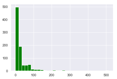
• Max fare seems an outlier

#Describe categorical features
titanic.describe(include=['O'])

	Name	Sex	Ticket	Cabin	Embarked
count	891	891	891	204	889
unique	891	2	681	147	3
top	Thomas, Master. Assad Alexander	male	347082	C23 C25 C27	S
freq	1	577	7	4	644

Observations:

• We can assume that name holds no significance in the survival of a passenger, hence we will drop this column
• Sex will be included in our predictions
• Looks like some people were sharing tickets. We will drop this column as well as it doesn’t show any significance
• Cabin seems to have alot of null values. We will drop it as well
• Embarked will be used in predictions

Exploratory data analysis

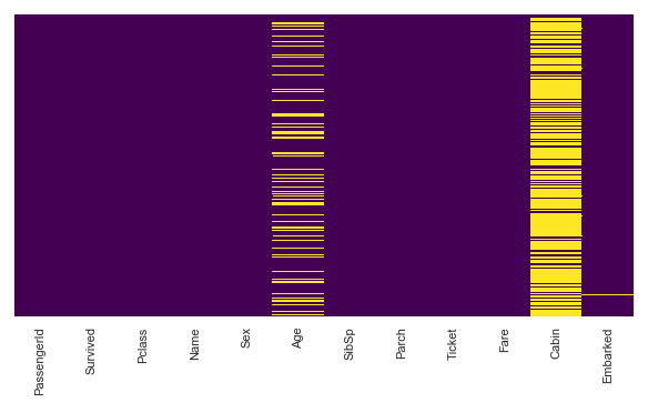
#Lets check for null values
plt.figure(figsize=(10,5))
sns.heatmap(titanic.isnull(),cbar=False,yticklabels=False,cmap='viridis')

    <matplotlib.axes._subplots.AxesSubplot at 0x28dd1756940>

[col for col in titanic.columns if titanic[col].isnull().any()]

    ['Age', 'Cabin', 'Embarked']

#We will drop cabin column as it has alot of null values. Dropping all unnecessary columns
titanic.drop(['Cabin','PassengerId','Name','Ticket'],axis=1,inplace=True)

We will impute the Age and Embarked columns later.

sns.countplot(x=titanic['Survived'],data=titanic,hue='Sex')

    <matplotlib.axes._subplots.AxesSubplot at 0x28dd1ab0978>

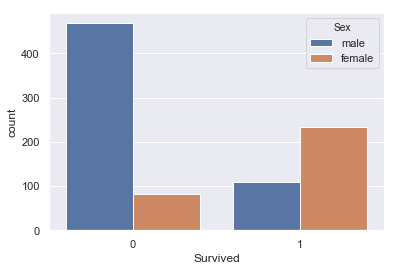
Looks like there were more female survivors.

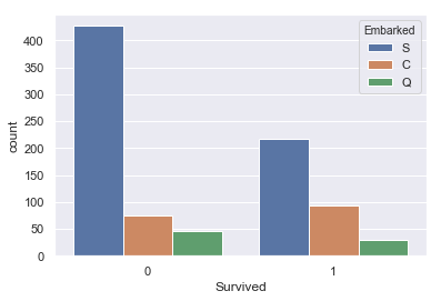
sns.countplot(x=titanic['Survived'],data=titanic,hue='Embarked')

    <matplotlib.axes._subplots.AxesSubplot at 0x28dd1b03278>

sns.countplot(x=titanic['Survived'],data=titanic,hue='Pclass')

    <matplotlib.axes._subplots.AxesSubplot at 0x28dd1b69470>

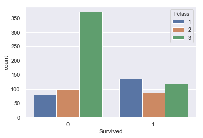
Looks like, people from 3rd class died more. Also, survival rate of 1st class is, somewhat, more than the other classes.

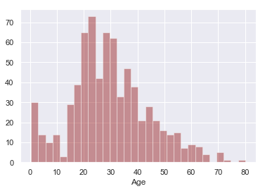
sns.distplot(titanic['Age'].dropna(),kde=False,color='darkred',bins=30)

    <matplotlib.axes._subplots.AxesSubplot at 0x28dd1bd1c18>

g = sns.FacetGrid(titanic,col='Survived',row='Sex')
g.map(plt.hist,'Age')

    <seaborn.axisgrid.FacetGrid at 0x28dd1add160>

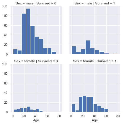
More infants survived. Also, 80 years old guy survived.

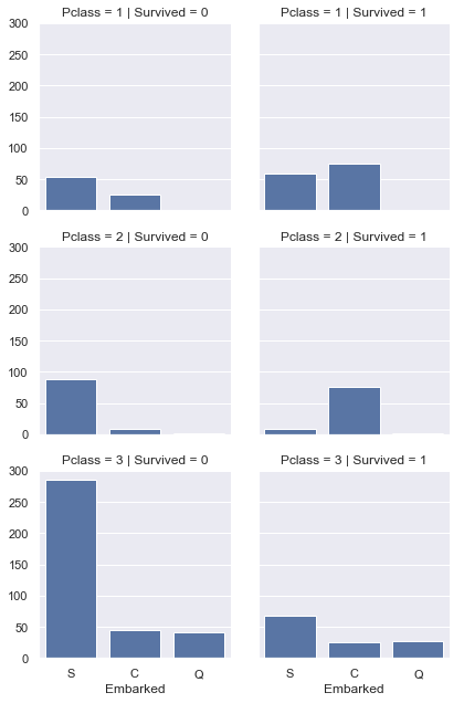
g = sns.FacetGrid(titanic,col='Survived',row='Pclass')
g.map(sns.countplot,'Embarked')

    <seaborn.axisgrid.FacetGrid at 0x28dd1c6df60>

titanic['Fare'].hist(bins=30,color='green')
    <matplotlib.axes._subplots.AxesSubplot at 0x28dd2155c50>

Pipelines

from sklearn.impute import SimpleImputer
from sklearn.preprocessing import OneHotEncoder
from sklearn.pipeline import Pipeline
from sklearn.compose import ColumnTransformer

#Separate target from predictors
X = titanic.drop('Survived',axis=1)
y = titanic['Survived']

#Lets separate the numerical and categorical columns
num_cols = [col for col in X.columns if titanic[col].dtype in ['int64','float64']]
cat_cols = [col for col in X.columns if titanic[col].dtype == 'object']

#Numerical transformer
num_transformer = SimpleImputer(strategy='mean')

#Categorical transformer
cat_transformer = Pipeline(steps=[
    ('impute',SimpleImputer(strategy='most_frequent')),
    ('onehot',OneHotEncoder(handle_unknown='ignore',sparse=False))
])

preprocessor = ColumnTransformer(transformers=[
    ('num',num_transformer,num_cols),
    ('cat',cat_transformer,cat_cols)
])

Get Model

from sklearn.linear_model import LogisticRegression
from sklearn.ensemble import RandomForestClassifier

model1 = LogisticRegression(solver='liblinear',random_state=1)
model2 = RandomForestClassifier(n_estimators=250,random_state=1)

#Model1 pipeline
final_pipeline_1 = Pipeline(steps=[
    ('preprocessor',preprocessor),
    ('model',model1)
])

#Model2 pipeline
final_pipeline_2 = Pipeline(steps=[
    ('preprocessor',preprocessor),
    ('model',model2)
])

Cross-Validation scores

from sklearn.model_selection import cross_val_score

scores_1 = cross_val_score(final_pipeline_1,X,y,cv=5,scoring='accuracy')

scores_1.mean()

    0.7912852282814269

scores_2 = cross_val_score(final_pipeline_2,X,y,cv=5,scoring='accuracy')

scores_2.mean()

    0.8115290623015141

We have achieved an accuracy of around 81% using RandomForest model.

XGBoost

from xgboost import XGBClassifier,XGBRFClassifier
from sklearn.model_selection import train_test_split

X_train, X_valid, y_train, y_valid = train_test_split(X, y, test_size=0.2, random_state=1)

model_XGBClassifier = XGBClassifier(n_estimators=1000, learning_rate=0.05, n_jobs=4)

model_XGBRClassifier = XGBRFClassifier(n_estimators=1000, learning_rate=0.05, n_jobs=4)

#Pipeline #1
pipeline_XGB = Pipeline(steps=[
    ('preprocessor',preprocessor),
    ('model',model_XGBClassifier)
])

#Pipeline #2
pipeline_XGBRF = Pipeline(steps=[
    ('preprocessor',preprocessor),
    ('model',model_XGBRClassifier)
])

params = {'model__early_stopping_rounds':5,
          'model__verbose':False,
          'model__eval_set':[(X_valid,y_valid)]}

scores_XGB = cross_val_score(pipeline_XGB,X_train,y_train,cv=5,scoring='accuracy')

scores_XGB.mean()

    0.8020450232017508

scores_XGBRF = cross_val_score(pipeline_XGBRF,X_train,y_train,cv=5,scoring='accuracy')

scores_XGBRF.mean()

    0.8356706923083909

Using the RandomForest flavor of XGBoost, we were able to achieve the accuracy of around 83.5%.