Bias Variance Tradeoff

We are going to understand the conecpt of Bias-Variance tradeoff in ML aka underfitting or overfitting your model.

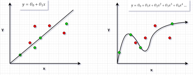
In the figure above, green dots are your training data and red dots are your testing data. We always fit our model with the training data. There are multiple ways to fit the green dots. One way is to fit a linear line through it (left figure). We can clearly see that it is not that good of a fit as most of the green dots have been missed by it let alone your testing data i.e. red dots.
The other way to fit green dots is by increasing your features and trying to fit the higher order polynomial like we did in the right figure. By increasing the complexity we can go as squiggly as possible so and so that we pass thourgh every green dot.

There is a problem with both the approaches. The left approach doesn’t fit even the training data completely. When your model doesn’t even fit the training data, it is said to be Underfitting or High Bias Alternatively, on the right is the approach where we fit the training data (green dots) perfectly but we will never be able to fit the red dots as the relation is too squiggly. When your model fits the training data perfectly but there is very high variance in predictions with test data, we call it Overfitting or High Variance

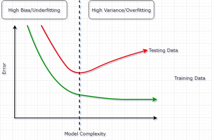
In the figure above, we can see that as we go to the right, our model gets more and more complex (same as we showed with fig 1 above on the right, we went upto 4th order of polynomial to fit the green dots) and our error rate drops on the training data (green line), however, error rate increases on the test data (red line).
Alternatively, if we stay on the left of the graph, our model will be very simple (like in fig 1 above on the left, we had a simple linear line) but we weren’t even able to pass the green dots completely.
We have to find that sweet spot somewhere in between (the dotted line above). The struggle of finding that sweet spot is known as bias-variance tradeoff.