Linear Regression and Gradient Descent

Supervised machine learning can be divided into:

• Regression
• Classification

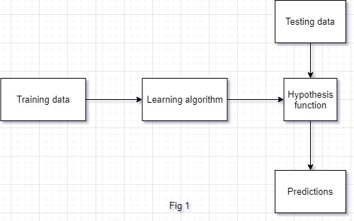
Today we will discuss the Linear regression models and the importance of Gradient descent. Our linear models works in a simple flow shown below in Fig 1. You train your model with the training dataset and the model will try to generate a hypothesis function \(h( x)\) that we can use to predict future values.

Univariate Linear Regression

To understand the concept fully, we will be discussing the regression with single variable also known as univariate linear regression.
Suppose you want to predict the price of a car based on it’s different features. For now we will be only taking one feature of car into consideration, lets say power of car. So in this case our independent variable (x) will be power of car and our hypothesis function \(h( x)\) will be the predicted prices of cars.

Our independent variable x (power of car in above example) is also known as feature, an ML lingo that we will use a lot.

Lets say we get data of 4 cars with their horsepowers and their prices and we feed this data to our learning algorithm. In response to that, our learning algo will try to generate a best possible hypothesis function \(h( x)\). We will display this in Fig 2 below:

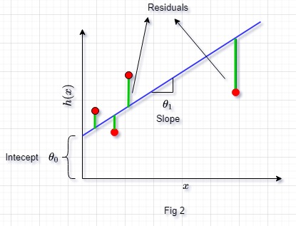
Red dots are the 4 cars data that we fed to our model. Blue line is our hypothesis function h(x), which shows the linear relation between the power of car and its price, that our model has come up with. We know from linear algebra, that we can represent the equation of this straight blue line as \(h( x) =\theta _{0} +\theta _{1} x\), where \(\theta_{0}\) is the y intercept and \(\theta_{1}\) is the slope of this line.

We can see that our predicted prices (i.e. blue line) doesn’t pass through the red dots which means that there is a difference between the actual prices of cars and the predicted prices. This difference between the actual values and the predicted values in known as Residuals (green lines).

But the question is how does our model know that which line to come up with, i mean there can be million straight lines that we can come up with but the question is which is the best one ?
Thats where two things come into play:

• Mean squared error (MSE) and
• Gradient Descent

Mean Squared error (cost) function

Lets define our cost function or MSE function as:

\[J( \theta ) \ =\ \frac{1}{2m}\sum\limits ^{m}_{i=1}( \ predicted\ value\ -\ actual\ value)^{2} \ =\ \frac{1}{2m}\sum ^{m}_{i=1}( h( x_{i}) \ -\ y)^{2}\]

Replacing our hypothesis function will give us:

\[J( \theta ) \ =\ \frac{1}{2m}\sum ^{m}_{i=1}( \theta _{0} +\theta _{1} x_{i} \ -\ y)^{2}\]

• \(m\) is the total number of training examples in our dataset which in our case is 4 as we took the data of 4 cars
• \(h(x)\) is the predicted price of car
• \(y\) is the actual price of car

We square the function to avoid the cancellation of positive residuals with negative residuals. Since this is the mean squared error, we divide it with the total number of training examples.

Also we have halved the total mean which will help us in future calculations and also halving the result won’t impact our calculations and in the end, we can always multiply the final result with 2 back again if we have to.

The whole purpose of our learning algorithm is to come up with a line that has the minimum value of our cost/MSE function \(J(\theta)\). So out of those million lines, it will pick the one that has the minimum value of our cost function

\[Goal:\ Minimize\ J( \theta )\]

In Fig 2, we can see that there are two variables to control our line \(\theta_{0}\) and \(\theta_{1}\)

By choosing different values of these two variables, we can come up with million different lines. Now our goal is to choose those values of these two variables that will give us the minimum value of our cost function \(J(\theta )\). Those values of \(\theta_{0}\) and \(\theta_{1}\) once placed inside our hypothesis function will give us the best possible line for our training dataset.

Now the question is, out of million possible values of \(\theta_{0}\) and \(\theta_{1}\), which values to choose. This is where the Gradient descent comes into action.

Gradient Descent

To grasp the concept of gradient descent fully, we will set \(\theta_{0}\) as 0 so that our cost function \(J(\theta)\) is a function of a single variable \(\theta _{1}\). We can now easily plot \(J(\theta)\) vs \(\theta_{1}\) in two dimensional space.

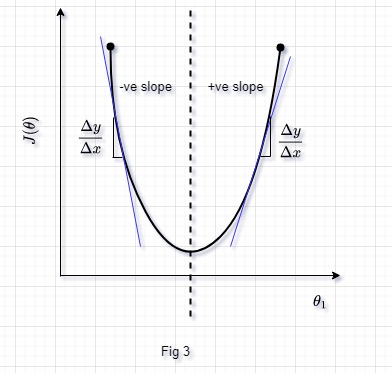
We have a parabola shape. These types of functions are also known as convex functions. They don’t have any local minimas or maximas, they only have global minima or maxima. We can see that in the figure as well, we have only global minima. The purpose of our gradient descent is to find that global minima, and that is the point where our cost function \(J(\theta)\) will have its minimum value.

Our gradient descent algorithm is:

\[\theta _{j} \ =\theta _{j} -\alpha \frac{\partial }{\partial \theta _{j}} J( \theta ) \ \ \ j=0,1,2,3...\]

• \(\alpha\) is the learning rate which controls the speed of gradient descent convergence
• \(\frac{\partial }{\partial \theta _{j}}\) is the partial derivative w.r.t. \(\theta\)

In case of our example with only single variable \(\theta_{1}\), our equation would be:

\[\theta _{1} \ =\theta _{1} -\alpha \frac{d}{d( \theta )} J( \theta )\]

Going back to our Fig 3, if we keep our learning rate \(\alpha\) constant and start the gradient descent algorithm with any value of \(\theta\) on the left of the dotted line. To find the derivate at any point, we would have to draw the tangent line at that point (blue line in Fig 3) and find its slope. We can see that the slope on the left of dotted line is always going to be -ve. Placing the -ve value in our above equation, we will get \(\theta _{1} \ =\theta _{1} \ +\alpha ( slope\ of\ tangent\ line)\), this will give us a positive value of \(\theta_{1}\) and hence our \(\theta_{1}\) will move towards the right.
Assume we start on the right side of the dotted line in Fig 3. Here derivative of tangent will always be positive, and our equation will become \(\theta _{1} \ =\theta _{1} \ -\alpha ( slope\ of\ tangent\ line)\). Hence our final value of \(\theta_{1}\) will decrease making us move towards the left in Fig 3.

We can keep our learning rate \(\alpha\) always fixed and our gradient descent equation will still converge to the global minima. But we have to make sure that we don’t use a very high value of \(\alpha\), else gradient descent will fail to converge or it may even diverge.

Gradient descent for Linear regression

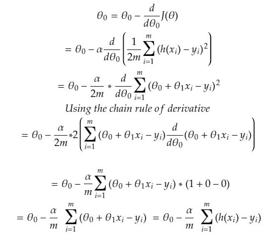
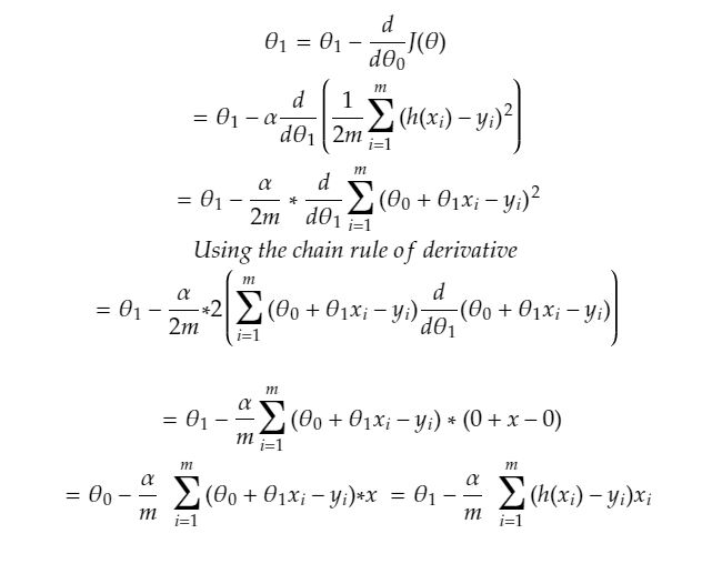
Replacing our linear regression’s cost/MSE function in the gradient descent equation above and solving for the two equations \(\theta_{0}\) and \(\theta_{1}\)

Solving for \(\theta_{1}\) :

Multivariate linear regression

The good thing about linear algebra is that whatever we conclude for two dimensions, we can map the same concept to more than 2 dimensions. Lets build our hypothesis function and gradient descent equations for n dimensions

\[h( x) =\theta _{0} x_{0} +\theta _{1} x_{1} +\theta _{2} x_{2} +....+\theta _{n} x_{n}\]

Let \(\theta\) and \(x\) be two vectors

\[\displaystyle \theta =\begin{bmatrix} \theta _{0}\\ \theta _{1}\\ .\\ .\\ \theta _{n} \end{bmatrix} \displaystyle x=\begin{bmatrix} x_{0}\\ x_{1}\\ .\\ .\\ x_{n} \end{bmatrix}\]

We can write our hypothesis function as:

\[h( x) =\theta ^{T} x\]

Our gradient descent with multivariate linear regression can be generalized as:

\[\displaystyle \theta _{j} =\theta _{j} -\frac{\alpha }{m}\sum ^{m}_{i=1}\left(\sum ^{n}_{j=0} \theta ^{( i) T}_{j} x^{( i)}_{j} -y^{( i)}\right) .x^{( i)}_{j}\]

or we can simply write

\[\theta _{j} =\theta _{j} -\frac{\alpha }{m}\sum ^{m}_{i=1}\left( h\left( x^{( i)}\right) -y^{( i)}\right) .x^{( i)}_{j} \ \ \ \ j=0,1,2,3....n\]

Do note that we have included \(x_{0}\) just to make our both vectors of same size i.e. \(n+1\). Value of \(x_{0}\) will always be 1.
Here \(m\) is the total number of training set examples and \(n\) is the total number of features per training example.

Credits: I would like to give the credit to Andrew Ng for his awesome course. If you like reading this article, go and enroll yourself in this course, you will love it.