Reaffirming the Central Limit Theorem

A very powerful concept in statistics is the Central limit theorem which states that if we have a population with mean \(\mu\) and standard deviation \(\sigma\), whether the population is normally distributed or not, if we collect a large number of samples from this population and take their mean, we would have that sample set’s mean. Then we take another set of sample from the same population and measure its mean, we would have another sample mean. If we do this again and again for a lot of sets of samples and each time the number of samples n that we collect is quite large, we would have many sample means with us. Central limit theorem states that when we plot that set of sample means, we would have a normal distribution with mean very close to population mean \(\mu\) and standard deviation of \(\sigma /\sqrt{n}\)

In statistics, we turn to normal distribution as much as possible as the calculations become a lot easier, thats why this theorem is super useful.

import numpy as np
import pandas as pd

import matplotlib.pyplot as plt
import seaborn as sns

%matplotlib inline
sns.set()

# Lets generate a random large population from a uniform distribution. I want to show the power of central limit theorem on non-normal distributions
population = pd.DataFrame()
population['Data'] = np.random.uniform(low=1, high=100, size=1000)

# Population mean
pop_mean = round(population['Data'].mean(), 1)
# Population variance
pop_var = round(population['Data'].var(ddof=0), 1)
# Population standard deviation
pop_std = round(np.sqrt(pop_var), 1)
print(f'pop_mean:{pop_mean},\npop_var:{pop_var},\npop_std:{pop_std}')
    pop_mean: 51.8,
    pop_var: 843.5,
    pop_std: 29.0

# Let us now get a single set of sample from that population
sample = population.sample(n=10, replace=True)

# Let us now calculate the mean and standard deviation of that single set of sample
sam_mean = round(sample['Data'].mean(), 1)
sam_var = round(sample['Data'].var(), 1)
sam_std = round(np.sqrt(sam_var), 1)
print(f'sam_mean:{sam_mean},\nsam_var:{sam_var},\nsam_std:{sam_std}')
    sam_mean: 47.0,
    sam_var: 735.7,
    sam_std: 27.1

We can see that we have different population mean and standard deviation than sample. Let us now put our knowledge of Central Limit Theorem into action. Let us now collect a large set of samples from the population

# sample_sets is the total number of sample sets
sample_sets = 10000
# 100 in below is the number of samples per sample_set
sample_means = [population.sample(100, replace=True)['Data'].mean() for x in range(sample_sets)]

pd.DataFrame(sample_means).plot(kind='hist', bins=100, density=True)
<matplotlib.axes._subplots.AxesSubplot at 0x25125a5de10 >

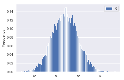
We can see that when we collect a very large set of samples, with a large samples per sample set, our distribution is pretty normal. Lets go ahead and find the mean and standard deviation of that distribution

round(pd.Series(sample_means).mean(), 1)
    51.9

which is almost our population mean 51.8

round(np.sqrt(pd.Series(sample_means).var(ddof=1)), 1)
    2.9

round(pop_std / np.sqrt(100))
    3.0

We can see that our standard deviation is very close to \(\sigma /\sqrt{n}\) which is according to the Central Limit Theorem

Applying Central limit theorem to Arbitrary distribution

We can go as arbitrary as possible and the results of central limit theorem would still be astonishing

population = pd.DataFrame([2, 8.9, 9.9, 1.3, 5, 19.5, 100, 34.5])

population[0].mean()
    22.6375

pop_std = np.sqrt(population[0].var(ddof=0))

pop_std
    30.981362845265537

sample_sets = 100000
sample_size = 1000
sample_means = [population.sample(sample_size, replace=True)[0].mean() for x in range(sample_sets)]

pd.DataFrame(sample_means).plot(kind='hist', bins=100, density=True)
    <matplotlib.axes._subplots.AxesSubplot at 0x2519b4f16a0 >

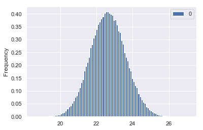
Awesome, we got another normal distribution. Let’s find out the mean and standard deviation of the sample mean distribution

pd.Series(sample_means).mean()
    22.631865978000167

which is exactly 22.63 as of our population mean

np.sqrt(pd.Series(sample_means).var(ddof=1))
    0.9756774327012292

pop_std / np.sqrt(sample_size)
    0.9797167160715387

This reaffirms our Central Limit theorem visually.